The Thrilling Thermo Field Dynamics and Its Special Applications (2024)

This article will discuss thermo field dynamics (TFD) and representations of various density operators in the TFD notation.

What is thermo field dynamics?

Thermo field dynamics is a theoretical framework designed for applications to quantum field theories at finite temperatures. Previously, it was used to find the exact solution to certain master equations encountered in Quantum Optics. In thermo field dynamics, we extend the given Hilbert space \(H\) to \(H \otimes {H^*}\) by taking the direct product of \(H\) with its dual \( {H^*}\). The main advantage of thermo field dynamics is that we can represent the operators defined in Hilbert space \(H\) by vectors in the extended Hilbert space \(H \otimes {H^*}\).

Consider an orthonormal basis\( |N\rangle \) defined in the Hilbert space \(H\). Then, any operator \(A\) on Hilbert space \(H\) can be expressed in terms of operators \({ |N\rangle \langle M| }\). In TFD (thermo field dynamics) notation, the same operator \(A\) can be represented as a vector in terms of basis vectors \({ |N, M\rangle }\) in \(H \otimes {H^*}\).

In thermo field dynamics, one assigns to every density operator \(\rho\) in \(H\), a vector \(|\rho^\alpha\rangle\) for \(0 \le \alpha \le 1\) in the extended Hilbert space \(H \otimes {H^*}\). Also, the quantum averages of the operators are expressible as scalar products:
\begin{equation}
\langle{A}\rangle = Tr({{\rho} {A}}) = \langle \rho^{1-\alpha} |A |\rho^\alpha\rangle \nonumber
\end{equation}
Where \(|\rho^\alpha\rangle = \hat{\rho^{\alpha}} |I\rangle\), with \(\hat{\rho^{\alpha}} = \rho^{\alpha} \otimes I \) and \( |I\rangle\) is the counterpart of the resolution of identity \(I\).

We can express \(I\) and \(|I\rangle\) as:
\begin{equation}
I = \sum_{N} |N\rangle \langle N| \nonumber
\end{equation}

In TFD:

\begin{equation}
|I\rangle = \sum_{N} |N,N\rangle
\end{equation}

Using the above formalism, we can assign a ket vector \(|\rho^\alpha\rangle\) to a density operator \(\rho\) defined in its own eigenbasis \(|K\rangle\) in the following way
\begin{equation}
\rho = \sum_{K} \rho_K |K\rangle \langle K|
\end{equation}

In TFD:

\begin{equation}
|\rho^\alpha\rangle = \sum_{K} {\rho}^{\alpha}_K |K,K\rangle
\end{equation}

In our examples in this article, we will deal with a harmonic oscillator coupled to a heat bath, of which the dynamics is dissipative, so we will use the representation of density operators in TFD notation with \(\alpha= 1\).

Quantum harmonic oscillator and thermo field dynamics

Since we will be dealing with harmonic oscillator states, which are Fock states, we can easily replace \(|N\rangle\) by \(|n\rangle\) and define creation and annihilation operators \(a^\dagger\), \(\tilde{a}^\dagger\), \(a\), and \(\tilde{a}\).
\begin{equation}
|n\rangle \langle m| \xrightarrow{TFD} |n,m\rangle \nonumber
\end{equation}
\begin{equation}
a|n,m\rangle = \sqrt{n}|n-1,m\rangle
\end{equation}

\begin{equation}
a^\dagger |n,m\rangle = \sqrt{n+1} |n+1,m\rangle
\end{equation}

\begin{equation}
\tilde{a} |n,m\rangle = \sqrt{m}|n,m-1\rangle
\end{equation}

\begin{equation}
\tilde{a}^\dagger |n,m\rangle = \sqrt{m+1} |n,m+1\rangle
\end{equation}

The operators \({a, a^\dagger } \in H\) and \({\tilde{a}, \tilde{a}^\dagger } \in H^{*}\), with \([a,a^{\dagger}] = [\tilde{a}, \tilde{a}^{\dagger}]= 1\) and \([a\hspace{2pt}\text{or}\hspace{2pt}a^{\dagger},\tilde{a}\hspace{2pt}\text{or}\hspace{2pt}\tilde{a}^{\dagger}] = 0 \).

From the above equations, we can easily see that-
\begin{equation}
a |I\rangle = \tilde{a}^{\dagger} |I\rangle, \hspace{25pt} a^{\dagger} |I\rangle= \tilde{a} |I\rangle \nonumber
\end{equation}

After this brief discussion of thermo field dynamics, we will discuss the representation of operators and some density operators in the TFD notation.

Consider an operator defined in the terms of operators \( |m\rangle \langle n| \) as
\begin{equation}
O = \sum_{m,n} O_{mn} |m\rangle \langle n| \nonumber
\end{equation}
In TFD notation, it can be represented as:
\begin{equation}
|O\rangle = \sum_{m,n} O_{mn} \frac{ {a^{\dagger m}} \tilde{a}^{\dagger n} }{\sqrt{m!n!}} |0,0\rangle \nonumber
\end{equation}
Now, we can discuss the TFD notation of some familiar harmonic oscillator states, such as single-mode thermal state and displaced single-mode thermal state.

Single-mode thermal state –

The expression for a single-mode thermal state is as follows:
\begin{equation}
\rho_{o} = (1-f)e^{-\beta a^{\dagger} a}
\end{equation}

$$ \text{With}\hspace{5pt} f = e^{-\beta}\hspace{5pt}\text{and}\hspace{5pt} \beta = \frac{\hbar \omega}{K_B T} $$
where \(K_B\) is Boltzmann constant, \(\omega\) and \(T\) are the frequency and temperature of the system. In TFD notation, the above state can be represented as

\begin{equation}
\begin{split}
\rho_o &= (1-f) \sum_{n} e^{-\beta n}|n\rangle \langle n| \\
|\rho_o\rangle &= (1-f) \sum_{n} e^{-\beta n} |n,n\rangle \\
|\rho_o\rangle &= (1-f) e^{f K_{+}} |o,o\rangle
\end{split}
\end{equation}

where \(K_{+} = a^{\dagger} \tilde{a}^{\dagger}\)

Displaced single-mode thermal state –

The expression for a displaced single-mode thermal state is as follows:
\begin{equation}
\rho_D = D(\alpha) {\rho_o} D^{\dagger}(\alpha) \nonumber
\end{equation}

where \(D(\alpha)\) is a displacement operator with \(\alpha\) as a complex number. In TFD notation, the above state can be represented as

$$ |\rho_D\rangle = D(\alpha)\tilde{D}(\alpha^*) |\rho_o\rangle $$

$$ |\rho_D\rangle = (1-f) D(\alpha)\tilde{D}(\alpha^*) e^{f K_{+}} |0,0\rangle $$

Where \(D(\alpha)=e^{\alpha a^{\dagger} – \alpha^* a}\).

Thermo Field Dynamics can help to find unique closed-form solutions-

Now we discuss the application of thermo field dynamics (TFD) to find a closed-form solution to a common term that usually appears when dealing with quantum physics, specifically quantum optics. Thermo field dynamics is a theoretical framework designed for applications to quantum field theories at finite temperatures.

Previously, it was used to find the exact solution to certain master equations encountered in Quantum Optics. In thermo field dynamics, we extend the given Hilbert space H to H⊗H∗ by taking the direct product of H with its dual H∗. The main advantage of thermo field dynamics is that we can represent the operators defined in Hilbert space H by vectors in the extended Hilbert space H⊗H∗.

We are going to find a closed-form solution to the term \( Tr[\Lambda^{a^\dagger a} D(\alpha) W_\beta D^\dagger(\alpha)] \) using thermofield dynamics by just utilizing the method to write gaussian states as vectors – in the context of a single quantum harmonic oscillator. For simplification, we denote this term as F[n] – the meaning will become clear as we proceed. The terms appearing in \(F[n] \) are the following:

The displacement operator, denoted by D(α), is represented by the formula \( D(\alpha) = e^{\alpha a^\dagger – \alpha^* a} \)

Thermal state: \( W_\beta = (1-e^{-\beta}) e^{-\beta a^\dagger a}\)

The parameter represented by the symbol \( \Lambda \) is a real number. Another restriction on \( \Lambda \) is that its value lies in the interval [0,1).

To start with we can express the term \( F[n] \) in the summation form as:

$$ F[n] = \sum_n \Lambda^n \langle n | D(\alpha) W_\beta D^\dagger(\alpha) | n \rangle $$

$$ F[n] = Tr[\Lambda^{a^\dagger a} D(\alpha) W_\beta D^\dagger(\alpha)] $$

Considering the dissipative dynamics of a harmonic oscillator, which allows us to set the parameter \( \alpha = 1 \) while writing the representation of any density operator in thermo field dynamics.

$$ Tr[\Lambda^{a^\dagger a} D(\alpha) W_\beta D^\dagger(\alpha)] = \langle \Lambda^{a^\dagger a} | D(\alpha) W_\beta D^\dagger(\alpha) \rangle$$

Where the term \( \bar{n} \) is the mean photon number of the thermal part of the displaced thermal state. Similarly, the other term inside the trace can be represented in thermo field dynamics as follows:

$$ | \Lambda^{a^\dagger a} \rangle = \frac{1}{1-\Lambda} e^{\bar{n}_\Lambda (K_+ + K_- – 2K_3)} | 0,0 \rangle $$

With \( \bar{n}_\Lambda = \frac{\Lambda}{1 – \Lambda} \) – This unique method to express the given operator as a thermal state in TFD is only possible due to the special restrictions provided on \( \Lambda \).

So $$ \langle \Lambda^{a^\dagger a} | = \frac{1}{1-\Lambda} \langle 0,0 | e^{\bar{n}_\Lambda (K_+ + K_- – 2K_3)} $$

$$ \langle \Lambda^{a^\dagger a} | D(\alpha) W_\beta D^\dagger(\alpha) \rangle = \frac{1}{1-\Lambda} \langle0,0| e^{(\bar{n} + \bar{n}_\Lambda) (K_+ + K_- – 2K_3) } | \alpha, \alpha^* \rangle $$

$$ \langle \Lambda^{a^\dagger a} | D(\alpha) W_\beta D^\dagger(\alpha) \rangle = \frac{1}{1-\Lambda} \sum_n \frac{(\bar{n} + \bar{n}_\Lambda)^n}{(1 +\bar{n} + \bar{n}_\Lambda)^{1+n}} e^{-|\alpha|^2} \frac{|\alpha|^{2n} }{n!}$$

$$ \langle \Lambda^{a^\dagger a} | D(\alpha) W_\beta D^\dagger(\alpha) \rangle = \frac{e^{-|\alpha|^2}}{(1-\Lambda)(1 +\bar{n} + \bar{n}_\Lambda)} e^{ \frac{(\bar{n} + \bar{n}_\Lambda)|\alpha|^{2}}{(1 +\bar{n} + \bar{n}_\Lambda)}} $$

$$ \sum_n \Lambda^n \langle n | D(\alpha) W_\beta D^\dagger(\alpha) | n \rangle = – \frac{ e^{ -\frac{ |\alpha|^2 (\Lambda – 1) }{ -1 + \bar{n}(\Lambda -1) } } }{ -1 + \bar{n}(\Lambda – 1) } $$

The exact evaluation of the discrete summation F[n] vs the closed-form expression plot shows that the solution is perfectly accurate.

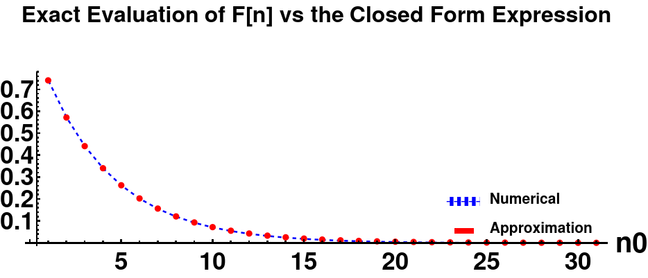
The figure above was generated using values of \( \bar{n} = 1 \) and \( \Lambda = 0.65 \).

The above-closed form expression of the given discrete summation is only valid when the parameter \( \Lambda \in [0,1) \). We hope the above analysis can be extended to find a closed-form solution using thermo field dynamics for complex cases of \( \Lambda \). We hope you enjoyed this proof while going through the equations.

Frequently asked questions

References:

Chaturvedi, S. (1993). Thermo field Dynamics and its Applications to Quantum Optics. In: Inguva, R. (eds) Recent Developments in Quantum Optics.

Thermo Field Dynamics and Condensed States

Quantum phase space distributions in thermofield dynamics J. Phys. A: Math. Gen. 32 1909

You might be interested in more articles on:

https://quantumthermodynamic.com