This article explains quantum entanglement in time. We all know that quantum entanglement in space refers to two particles that are separated in space and can influence the physical description of each other when measured. The question arises here of whether something similar is also possible across time. In this article, we will discuss a research paper – “Entanglement Swapping between Photons that Have Never Coexisted”, that explains it.
|State of a Quantum System>
In classical physics, the state of a particle can be described by its position and momentum – which implies that a particle stays in a fixed state at a given time. In Quantum mechanics, a particle can exist in multiple states simultaneously. Mathematically, the state of a particle can be represented using Dirac notation.
Considering a two-level system as shown:
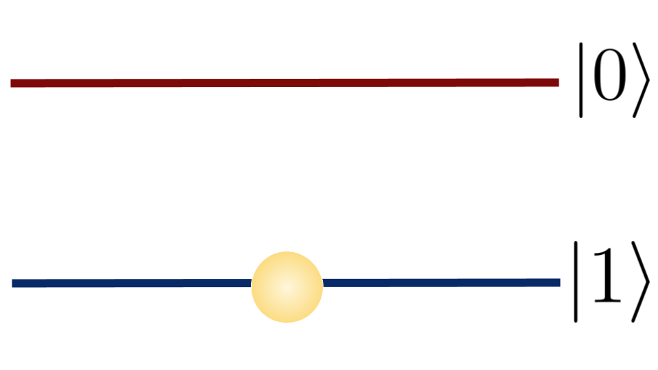
$$ |\Psi \rangle = \alpha |0\rangle + \beta |1\rangle $$
Such that the probabilities of being in that state add up to 1. It can be expressed as \( |\alpha|^2 + |\beta|^2 =1 \).
Quantum Entanglement in Space
Consider two classical macroscopic masses, X and Y, and let’s put them in two identical boxes and distribute them between Alice and Bob, who are in France and Germany, respectively. If Alice finds X, Bob will get Y and vice versa. Suppose we send the box with X to Alice and Y to Bob. Then, even if Alice or Bob does not open the box, we know that there is X in Alice’s box and Y in Bob’s box. When one of them opens their box, they will instantly know what is in the other box. But it is impossible that we send X to Alice, and when Alice opens the box, there is a 50% probability of getting X and a 50% probability of getting Y. In quantum mechanics, the case is different; a particle can exist in superpositions of states until its state is measured. All we want to learn from this paragraph is that its state is not deterministic until measured.
To understand Quantum entanglement, consider the decay of a particle into two other particles, which are travelling in opposite directions, and consider that these are spin \( \frac {1}{2} \) particles. Their state after decay can be represented as:
$$ | \Psi_{1,2} \rangle = \frac{1}{\sqrt{2}} ( |01\rangle + |10\rangle ) $$
Where \( |0\rangle \) implies Up spin \(+\frac{1}{2}\) and \( |1\rangle \) implies Down spin \(-\frac{1}{2}\). From the above state, we can see that if particle one is found in state \(|0\rangle\), then the second particle will be in state \(|1\rangle\) on measurement and vice versa.
The above example shows the quantum entanglement in space – where two particles are separated in space and are linked in a way such that measurement of the state of one particle affects the physical description of other particles’ state irrespective of the distance (in space) between them.
Quantum Entanglement in Time
In the example of quantum entanglement in space, we have seen that two particles separated in space can be linked to each other, but is it possible for two particles that do not coexist and be entangled – or in other words, is it possible that measurement performed on the state of one particle at some time can affect the physical description or the measurement of the state of other particles at different time. The answer is Yes!
In the article – “Entanglement Swapping between Photons that Have Never Coexisted”, the authors consider two pairs of photons generated with a time-gap of \( \tau \). First, the first pair of two Photons(1,2) is created at time \( t=0 \), and the first photon is measured immediately after it is created. After this, the second photon is delayed until the other pair of Photons (3,4) is created at time \( t = \tau \). After this, the second photon of the first pair and the first photon of the second pair, Photon 2 and Photon 3, are projected onto the bell basis. The second photon of the second pair is also delayed by \(\tau\) in a delay line.
The combined state of these four photons can be represented as:
$$ |\Psi^-\rangle_{1,2}^{0,0} \otimes |\Psi^-\rangle_{3,4}^{\tau,\tau} $$
Where we are using the definition of time-like bell states:
$$ |\Psi^\pm \rangle_{a,b}^{\tau,\tau’} = \frac{1}{\sqrt{2}} (|h_a^{\tau} v_b^{\tau’} \rangle \pm |v_a^{\tau} h_b^{\tau’} \rangle ) $$
$$ |\Phi^\pm \rangle_{a,b}^{\tau,\tau’} = \frac{1}{\sqrt{2}} (|h_a^{\tau} h_b^{\tau} \rangle \pm |v_a^{\tau} v_b^{\tau’} \rangle ) $$
After applying the given procedure, the final combined state is denoted as:
\begin{equation}
\begin{aligned}
|\Psi^-\rangle_{1,2}^{0,\tau} |\Psi^-\rangle_{3,4}^{\tau,2\tau} = \frac{1}{2} [ |\Psi^+\rangle_{1,4}^{0,2\tau} |\Psi^+\rangle_{2,3}^{\tau,\tau} – |\Psi^-\rangle_{1,4}^{0,2\tau} |\Psi^-\rangle_{2,3}^{\tau,\tau} -|\Phi^+\rangle_{1,4}^{0,2\tau} |\Phi^+\rangle_{2,3}^{\tau,\tau} + |\Phi^-\rangle_{1,4}^{0,2\tau} |\Phi^-\rangle_{2,3}^{\tau,\tau} ]
\end{aligned}
\end{equation}
We can do a bit of mathematics to see how the above state can be written in the given form. From the definition of time-like bell states, we can write:
\begin{equation}
\begin{aligned}
|\Psi^-\rangle_{1,2}^{0,\tau} |\Psi^-\rangle_{3,4}^{\tau,2\tau} &= \frac{1}{2} (| h_1^0 v_2^\tau \rangle – | v_1^0 h_2^\tau \rangle) \otimes (| h_3^\tau v_4^{2\tau} \rangle – | v_3^\tau h_4^{2\tau} \rangle)
\end{aligned}
\end{equation}
If we project Photon 2 and Photon 3 in the above state onto a bell state \( | \Psi^{+}_{2,3} \rangle \), then I can be expressed in the following way:
$$ \langle \Psi^{+}|_{2,3}^{\tau,\tau} [|\Psi^-\rangle_{1,2}^{0,\tau} |\Psi^-\rangle_{3,4}^{\tau,2 \tau}] | \Psi^{+} \rangle_{2,3}^{\tau,\tau} = \frac{1}{2} | \Psi^+ \rangle_{1,4}^{0,2 \tau} | \Psi^{+} \rangle_{2,3}^{\tau,\tau} $$
Similarly, other terms can be calculated. From the above term, we can see that if Photon 2 and Photon 3 are projected on state \( | \Psi^{+}_{2,3} \rangle\), then the resulting state of Photon 1 and 4 is:
$$ | \Psi^+ \rangle_{1,4}^{0,2 \tau} = \frac{1}{\sqrt{2}} ( | h_1^{0} v_4^{2\tau} \rangle + | v_1^{0} h_4^{2\tau} \rangle ) $$
We can see that after performing bell projection on Photons 2 and 3, Photons 1,4, which did not share any correlations between them, became entangled. This entanglement can be seen as entanglement between photons that do not coexist, and it is referred to as Quantum entanglement in time.
References:
[1] Entanglement Swapping between Photons that have Never Coexisted
E. Megidish, A. Halevy, T. Shacham, T. Dvir, L. Dovrat, and H. S. Eisenberg
Phys. Rev. Lett. 110, 210403 – Published 22 May 2013
https://journals.aps.org/prl/abstract/10.1103/PhysRevLett.110.210403
If you like reading it, then share the link on social media – https://quantumthermodynamic.com/quantum-entanglement-in-time/